
The satellite industry is full of people, myself included, who do not have backgrounds in Engineering. For those of us who fall into this camp the specifications for radio-frequency (RF) devices can be mysterious and intimidating—arcane symbols and abbreviations we do not understand and numbers whose significance eludes us.

If these challenges sound familiar to you then read on—the goal of this article is to review commonly-used specifications; to explain what they are and why they truly matter.
Before we move on, a comment on decibels (dB). A decibel is not really a unit of measurement like watts or volts or degrees. Rather, this is a unit used to quantify the ratio between two things (usually power or intensity) on a logarithmic scale.
The use of a logarithmic scale allows us to compare large and small numbers without a bunch of annoying zeros getting in the way. As a reference, 0 dB equates to 1, 10 dB equates to 10, 50 dB equates to 100,000 and 100 dB equates to 10,000,000,000. The key element to remember is the difference between two numbers that are both stated in dB can be quite a bit larger than such appears at first glance. This is a good to keep in mind when you are comparing specifications for different products. I recommend the Wikipedia article on decibel if you would like to read more information on this topic.
Let’s begin our adventure by looking at an attribute that I have found particularly challenging: voltage standing wave ratio (VSWR). A quick Google search defines VSWR as the ratio of the maximum RF voltage to the minimum RF voltage along the line. I’m sure this is meaningful to the Electrical Engineers in the crowd, but I do not find it to be a particularly illuminating explanation of what is going on.

For me, the easiest way to think about VSWR is as a way to quantify the efficiency of power transfer through a system. A perfectly efficient system would have a VSWR of 1:1—all of the power that enters the device would exit. This, of course, is not what happens. A certain amount of the power is always lost to inefficiencies.
The goal, of course, is to minimize this loss in order for as much power as possible to be delivered. VSWR is also a logarithmic scale; the difference between 2:1 and 4:1 may not seem that large, but in reality, 2:1 is pretty good and 4:1 would be practically unusable. VSWR is specified both at the input and output interfaces of a device.
Once you know what the VSWR is, you can use that ratio to calculate return loss, which is the loss of power caused by a discontinuity, such as the connector between two components, reflecting a portion of the power backwards into the system. Return loss is measured in dB, and counterintuitively, the greater the return loss is in decibels, the better. Note that for historical reasons, return loss is sometimes shown as a negative number. When this is the case, the measurement should be called reflection coefficient instead.
Conversion gain is a measure of the difference between the power of an input signal and the power of an output signal. Gain is given in dB, and larger numbers are better. Gain between 50 dB and 60 dB is generally considered sufficient for most satellite communication purposes.
In the case of LNBs (Low-Noise Block Downconverter), this means amplifying the very weak signals received from a satellite approximately 500 to 1,000 times so that they are sufficiently strong enough to be deciphered by a modem. In the case of a BUC or SSPA this means amplifying the power that is received into the device by approximately 500 to 1,000 times in order for the outgoing radio waves to have enough energy to reach their targeted satellites.
As you can imagine, this results in a great deal of energy and explains why it is unwise to stand in the path of a transmitting antenna.
In a perfect universe, gain would always be linear; the power coming out of a system would continue to increase at the same rate as the power going in and higher gain would always be better. Unfortunately, this is not the case. At some point, the output power begins to drop off relative to the input power and trying to increase gain past this point ultimately leads to distortion, saturation and ultimately damage to the device. A bit more on this topic will be presented later in this article.
Gain variation, or gain flatness, is a measurement of the difference in gain across the output frequency of a product and is measured in decibels peak-to-peak (dB p-p), either across the entire operating band of the device or over any 40 MHz (40 MHz is generally the bandwidth of a single satellite transponder). This can also be measured across a temperature gradient or over time. The closer this number is to zero, the better, as very low numbers mean you will witness consistent behavior of the device across its operating parameters.
Output power is one of the primary specifications for BUCs and SSPAs, which makes perfect sense as higher wattage products provide higher data rates and higher throughput. The cost of products increases as wattages get higher, and those costs can be quite high indeed for higher power units.
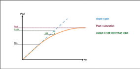
Unfortunately output power is also one of the most unclear specifications for these devices, mainly due to a lack of standards. Sometimes, especially for high-power Ku-band and for Ka-band products, power is specified at the amplifier’s saturation point: Psat. Sometimes power is specified at the point where there is a 1dB difference between the theoretical linear gain and the actual gain: P1dB. Sometimes power is specified at the point before gain deviates from linear: Plin.
There is no easy way to convert the output power at one of these points to output power at a different point. Any time you are comparing BUCs and SSPAs, read the specification sheets carefully to understand what the output power is at these three points. If this information is not in the spec sheet, ask the vendor to tell you; this is the only way you can be certain you are comparing apples with apples.
Note that power is not specified for LNBs. This is because the signal strength coming into the LNB is so very low that is not possible to saturate or over-drive the device during normal operations.
Local oscillator (L.O.) stability is also an important figure in LNB specifications as it determines what types of systems the LNB can be used in. To go back to basics, the function of an LNB within a system is to extract a signal of interest from the microwaves collected by the antenna, and then to amplify that signal and mix it with the L.O. frequency to create the output frequency that is then sent to the modem. If an LNB has a very high stability, for example +/- 2 kHz, the output frequency will not vary much at all. This means that the modem will reliably receive a very narrow band transmission, leaving adjacent frequency bands available for other uses.
Applications such as voice communications rely on this level of stability. If an LNB has a low L.O. stability, for example, of +/- 2000 kHz (2 GHz), the output frequency will vary considerably. In broadband applications such as HDTV transmission, this is not a problem, as the resulting output frequency will still be acceptable to the modem. Note that products with high L.O. stability are more expensive than those with low L.O. stability. External reference LNBs, which use a “locked” external signal that does not vary at all, are even more expensive. Which L.O. stability is “best” depends on the input requirements of the modem and what the intended use of the modem.
Noise is measured in dB and is caused by the unwanted electrical contributions of a device’s components. As one would guess, the closer to zero the noise figure is the better. This is especially important in LNBs as the strength of the signal received from the satellite is low enough that too much noise can completely overwhelm the signal. As an aside, there is an interesting challenge in RF design relative to noise: input circuits that are designed for low noise frequency tend to have higher VSWR and vice versa.
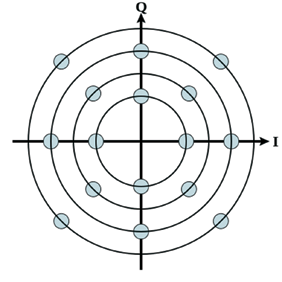
Phase noise is a particular subset of noise. It refers to random fluctuations created in the phase of a waveform, and can destroy the orthogonality (being at right angles to one another) of the signals. If this occurs, the polarization of the microwave path between a satellite and an antenna can be destroyed, making it impossible to determine which of the data streams a particular bit belongs to. Phase noise is measured in decibels relative to carrier per hertz (dBc/Hz), and large negative numbers are better than those closer to zero. Note that phase noise is more of a problem for low data rate transmissions such as voice than for high data rate transmissions such as HDTV as there is less ability for the modem to correct for lost bits.
Last, but not least, we have spurious. Spurious is my favorite specification, as it is a measurement of the strange things that happen as gain begins to go non-linear and power begins to misbehave. This misbehavior results in unwanted, in-band frequencies being generated within the system, causing distortion.
Spurious is measured in decibels relative to carrier (dBc) at the rated power for the product. A negative number, the further from zero the db is, the better. Note it is important you understand if the rated power is P1dB or Psat when you are looking at the spurious specifications that the difference between the theoretical linear gain and the actual gain curve is smaller at P1dB than it is at Psat, so there will be fewer peculiarities occurring at lower power levels.
There are, of course, other RF specifications that I have not covered, but I hope that this information I have provided will serve as a good base upon which you can build your knowledge and make wise product decisions.