
The coverage and capacity band of the new 5G cellular network will operate mostly at 3.3 to 3.6 GHz posing interference concerns with the C-band satellite communication terminals which receive Space-to-Earth signals in the 3.4 to 4.2 GHz band. In this article, we prove that the interference signal, in a worst-case scenario, could be orders of magnitude higher than what the C-band terminal can tolerate.
Possible solutions are investigated and the products presented that can mitigate the interference. These products include LNBs with built-in filters and waveguide filters each of which may be a standalone solution or be combined to provide greater rejection of the interference. Guidelines on how to locate the C-band terminals are also presented.
Introduction
Satellite communication terminals operate in different frequency bands, one of which is called C-band. Terminals operating in C-band normally receive signals in the range of 3.4 to 4.2 GHz and transmit signals in the range of 5.85 GHz to 6.425 GHz. Until recently, there was no other well-established terrestrial technology operating in this band.
Although some WiMAX and other terrestrial networks operated at similar bands, they were never widespread and did not raise serious interference concerns. However, 5G cellular technology is expected to be ubiquitous and will share the same spectrum. The 5G interference signals will be powerful enough to saturate the sensitive C-band satellite receiving systems, causing a potential for total loss of service.
To support the efficient coexistence of 5G and LTE operating in the same licensed frequency band, the 3.3 to 3.8 GHz band has gained popularity for developing the 5G network in the coverage and capacity layer [1], [2]. However, in many regions and countries the spectrum of the 5G networks will be limited to below 3.6 GHz such as in Russia, MENA, China, Africa. Some of these countries will also use the range 4.8 GHz to 5.0 GHz or frequencies above 4.4 GHz. In Europe, most countries are planning to use the 3.4 GHz to 3.8 GHz range [2].
As the above mentioned 5G frequency bands fall in the C-band receive spectrum of 3.4 GHz to 4.2 GHz, the receiver of a C-band terminal operating at the same frequency as the 5G signal will face interference. Even if the satellite signals received by the C-band terminal are limited to 3.8 to 4.2 GHz, there is still a risk of 5G signal interference. The satellite signal received at the ground terminal is usually several orders of magnitude weaker than the cellular signal. The receiver equipment of a satellite terminal is usually chosen or designed to detect these extremely low power levels in the 3.4 to 4.2 GHz range and the presence of any strong carrier may affect the performance of its receiving system including the LNB and the modem. These adverse effects, which may be experienced even if the interfering signal is out of band, include...
— Gain compression and saturation
— Noise floor degradation
— Unwanted Intermodulation products
Gain compression occurs when the total power at the input of the LNB reaches or passes its input P1dB. For example, an LNB with an output P1dB = 5 dBm and a gain of Gss = 60 dB will have an output at P1dB if the interfering signal is -54 dBm. This will occur even though the received satellite signal is very small and would not normally cause gain compression. An LNB operating with gain compression will lead to a non-linear distortion at the input of the modem which may affect the modulation error ratio (MER) and Eb/N0 and thus the bit error rate. In a worst-case scenario, the modem may lose the receive lock.
Saturation happens when the power in the interfering signal is too strong and forces the receiver into saturation. In the above example if the interference has a power of around -45 dBm or above, the LNB could be blocked and may not be able to receive any signals.
Noise floor degradation is another effect which may be either uniform across the entire receiving band of the LNB or only present at portions of it. If the noise floor is raised, the signal to noise ratio (C/N) and Eb/N0 will be reduced leading to an increase in the bit error rate.
Intermodulation will occur between the interfering signal and the satellite receive signal or between the interfering signal and the LO of the LNB. The frequency of the resulting intermodulation products could fall into, or close to the operating spectrum of the LNB and cause further interference or simply reduce the linearity of the LNB.
Although this article focuses on a specific interference problem which occurs at 3.6 GHz, the generality of this method remains intact and the reader can apply it to any frequency.
In this article, the received interference power in one near-field and one far-field worst case scenario are calculated and estimated and solutions are recommended to overcome the issue. Multiple interferers are not considered. The effects of multi-path are not considered.
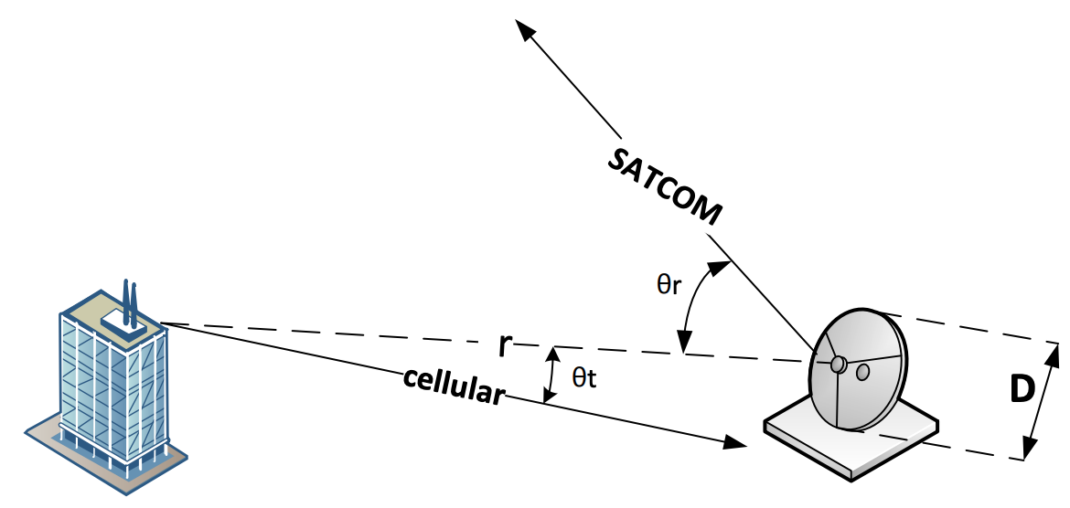
Figure 1. The dashed line shows the distance, r, between the cellular and SATCOM antennas. The line named "SATCOM" shows the boresight of the C-band reflector antenna, making angle with the dashed line. The line titled "cellular" shows the boresight of the cellular antenna making an angle with the dashed line. For simplicity and without loss of generality, all three lines are assumed to be on the same plane. The size of the dish is denoted by D.
5th Gen Cell Signal Interference with C-band SATCOM Terminals
Two worst-case scenarios are now presented wherein the interference from a 5G cellular antenna seems to be significant. The first case occurs at the distance from the antenna known as the far-field distance and the second case takes place when the interferer is closer to the antenna and thus the far-field approximations no longer apply. For simplicity, not accounted for are the multiple sources and the multipath effects.
The field values are calculated assuming 40 W radiation from a cellular antenna with a gain of 18 dBi [5]. Field values and power densities are calculated using standard far-field approximations and some near-field approximations [3] and [4]. The summary of the results are presented in the main body of this article, while the detailed calculations can be found in the Appendix.
As seen in Figure 1, the transmitting antenna in the defined problem is a cellular antenna whose radiation pattern is usually omnidirectional in the horizontal plane, meaning that its gain is not dependent on 𝜙𝑡. This is usually achieved by using several sector antennae, each of them covering a region. To be conservative, we assume that the receiving antenna is on the boresight of the transmitting antenna, making 𝜃𝑡 = 0, and thus maximizing the transmitted power density. The cellular antenna is in the far field region of the C-band SATCOM terminal if the distance 𝑟 is greater that the distance to the boundary of the far-field region denoted by 𝑅𝑓 which is dependent on the size of the antenna and the wavelength.
The free space loss and the power received by the C-band terminal is computed for different distances. According to [3] the highest power density in the near field occurs at 𝑅𝑓 /10 and so this is considered the worst-case scenario and is one of the distances we use for received power, 𝑃𝑟 , calculation. We also calculate 𝑃𝑟 at 𝑅𝑓 and 2𝑅𝑓 .
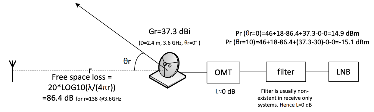 Figure 2. Link budget calculation for the interference caused by a cellular antenna and received by a 2.4- m reflector antenna at 138 meters away.
For a 2.4-m antenna at 3.6 GHz, 𝑅𝑓 is equal to 138 meters, therefore 𝑃𝑟 is calculated at 13.8 m, 138 m and 276 m. These calculations are performed assuming that the cellular antenna is at the boresight of C-band SATCOM terminal, that is 𝜃𝑟 = 0 which is an unlikely scenario as it may cause blockage to the line of sight to the satellite. However, they provide a baseline for further calculations such as when the cellular antenna is not at the boresight of the reflector antenna. The calculations are repeated for an offset angle of 𝜃𝑟 = 10 degrees.
All the calculations for a 2.4 m antenna at 3.6 GHz are summarized and illustrated in Figure 2.
The far-field distance 𝑅𝑓, free space loss, and 𝑃𝑟 are calculated again for different antenna sizes, both at boresight and at 𝜃𝑟 = 10 degrees. The results are summarized in Table 1.
The last two columns in Table 1 show the received interference levels for different antenna sizes at different distances, assuming both the unlikely case of 𝜃𝑟 = 0 and more likely case of 𝜃𝑟 = 10 deg. The boresight assumption is unlikely to occur as it may cause satellite blockage. The gain at 10-degree offset angle is obtained from the mask provided in FCC 25.209(a)2.
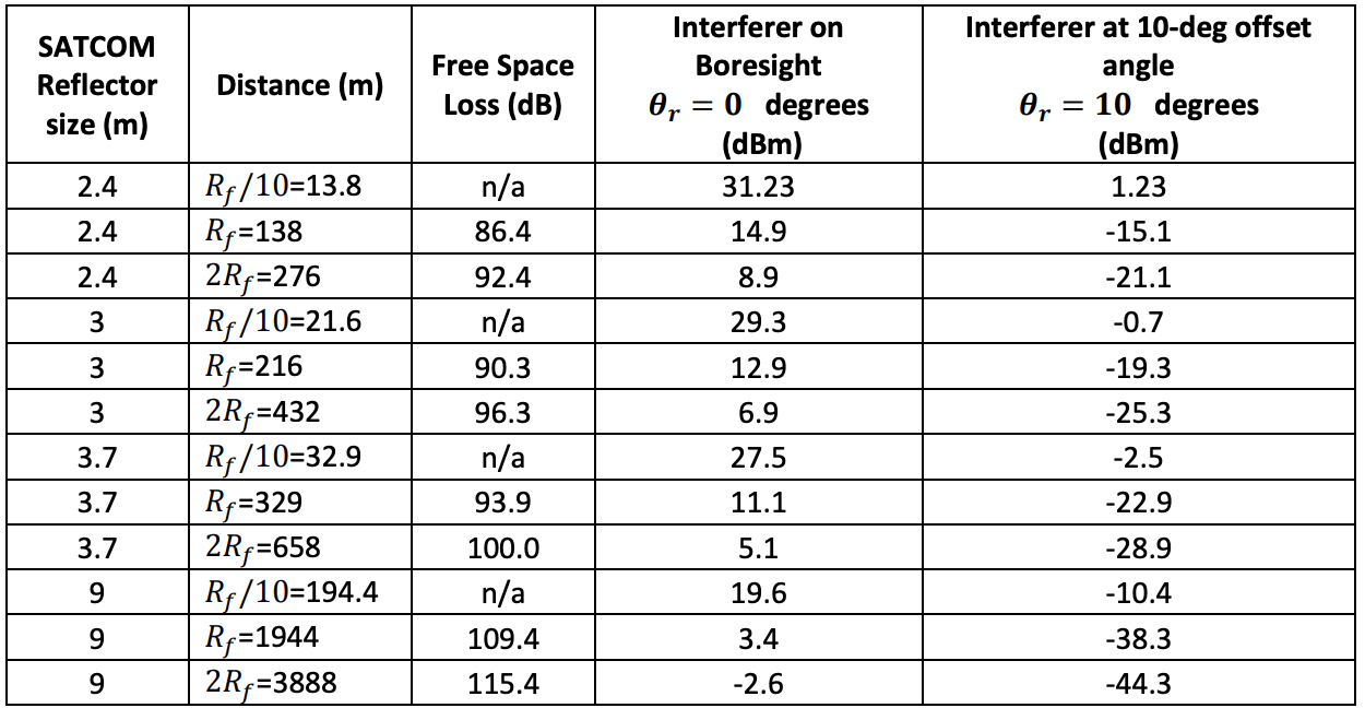 Table 1. Interference level received by reflector antennas of different sizes at 3.6 GHz caused by a 40 W cellular antenna with a gain of 18 dBi.
If the assumption is made that the interferer is always at least 10 degrees offset from reflector antenna bore-site and in the far field of the reflector antenna, i.e., ignoring the 𝑅𝑓/10 distances, it is seen that the interference level at the LNB input is always below -15 dBm.
Sensitivity of Standard C-band LNBs
Norsat conducted a series of tests to determine the immunity level of typical C-band LNBs which work in the 3.4 to 4.2 GHz range and hence innately susceptible to interference at 3.6 GHz.
The gain and noise floor of a standard LNB was measured, across the 3.8 to 4.2 GHz range with and without an interference signal at 3.6 GHz.
Figure 3 shows the standard LNB output when no interference signal is present. A -50-dBm signal at 3.6 GHz is used as the interference the output is presented in Figure 4 which shows intermodulation products.
Figure 1. The dashed line shows the distance, r, between the cellular and SATCOM antennas. The line named "SATCOM" shows the boresight of the C-band reflector antenna, making angle with the dashed line. The line titled "cellular" shows the boresight of the cellular antenna making an angle with the dashed line. For simplicity and without loss of generality, all three lines are assumed to be on the same plane. The size of the dish is denoted by D.
Figure 2. Link budget calculation for the interference caused by a cellular antenna and received by a 2.4- m reflector antenna at 138 meters away .
The intermodulation products almost disappear when the strength of the interference is below -55 dBm. Therefore, this is considered as the sensitivity of the standard LNB.
Unfortunately, all interference levels shown in Table 1 are above -55 dBm which indicates that a standard LNB will experience performance problems due to interference from a 5G cellular tower.
All the strategies that can be used to tackle the interference problem are reviewed in the following section.
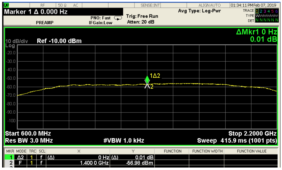 Figure 3. Output of a standard LNB with no interference.
Mitigating the Risk of Interference
To eliminate or control any electromagnetic interference one must focus on three major fronts -the transmitter, the medium of propagation and the receiver.
Transmitter
The power, the radiation pattern or the location of the 5G base station antenna cannot be controlled. Moreover, the antenna array of the 5G base station is usually designed to provide an omnidirectional radiation pattern in the horizontal plane. However, in the vertical plane, the radiation pattern is not uniform and has about 15 dB less gain at an offset of 15 degrees. As base station antennas are usually on buildings, the radiation patterns typically have a down-tilt to provide better coverage at ground level. If the satellite antenna can be located higher than the 5G antennas, it may be possible to benefit from the reduced gain of the 5G antenna in the direction of the satellite antenna. These estimates are dependent on the manufacturer of the sector antenna, its exact radiation pattern, the base station site and RF planning.
Medium of Propagation
The 5G signal power received by the satellite antenna decreases with the distance between the antennas. Assuming interferer is in the far field region of the satellite antenna, the received power density is reduced 7 6 dB each time the distance between the antennas is doubled. So whenever possible, choose the farthest distance from the base station antenna.
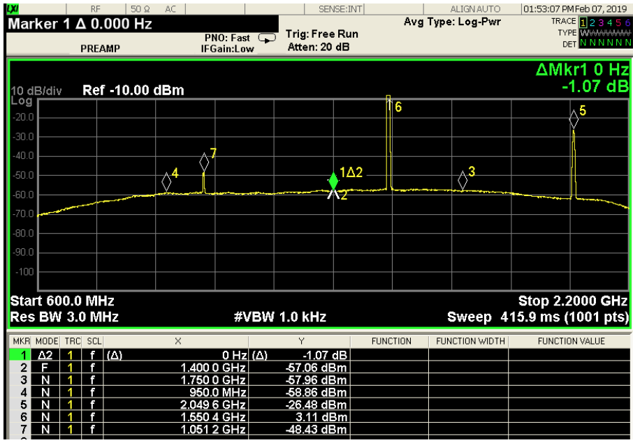 Figure 4. Output of a standard LNB with input CW interference at 3.6 GHz and power of -50 dBm.
Solutions at the Receiver
Position
Sometimes it is possible to locate the C-band terminal such that the base station antenna is at the widest possible offset angle from its boresight. The site of the C-band terminal can be analyzed to provide instructions as how to position the terminal in order to reduce the interference. The last column in Table 1 is an example of the effect of a 10-degree offset angle in reducing interference.
Interference Mitigating LNBs
A typical LNB tolerated an interference of -55 dBm at 3.6 GHz with minimal intermodulation or gain compression. However as shown previously, it is expected interfering signals may be as high as -15 dBm. A current design for an interference-mitigating LNB is expected to tolerate an interference of -20 dBm without any significant spurious or intermodulation products at the output. The cost of this additional interference tolerance is that the noise temperature is expected to increase from about 40 K to about 54 K.
Unfortunately using the interference-mitigating LNB does not eliminate the interference problem in all cases and some additional filtering before the LNB may be required. Table 2 summarizes the additional filtering that is required for various scenarios using a 2.4m antenna and the interference levels provided in Table 1.
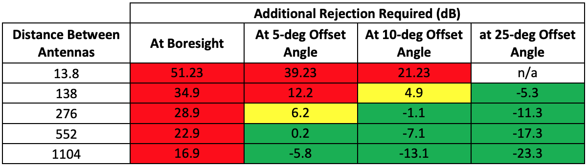 Table 2. Amount of additional rejection required (dB) in order to mitigate the interference while using a new interference-mitigating LNB. The green cells indicate the positions at which the new interference-mitigating LNB will definitely work as a standalone solution, assuming the conditions explained in the paper. The yellow cells indicate the positions at which the new interference-mitigating LNB will probably work at the actual gain pattern is usually several dB below the mask. The red cells indicate the situations where a waveguide filter is necessary.
It is seen in Table 2, that at a more likely 25-degree offset angle, at all far field distances the new interference-mitigating LNB is sufficient to mitigate the risk of interference. The gain at offset angles are obtained from the mask provided in FCC 25.209(a)2.
The actual radiation pattern of an antenna will usually have a gain of several dB lower than the mask at wide offset angles. Hence when the additional rejection required is about 6 dB or less, (i.e., the yellow cells in Table 2) it is expected that the interference-mitigating LNB by itself will be sufficient.
The red cells in Table 2 indicate the amount of additional rejection required when the interference-mitigating LNB does not mitigate the interference by itself. In these situations, a waveguide filter will be necessary.
Waveguide Filter
A waveguide filter can be used to suppress the frequency content at the interference band. The benefit of this method is that the interference is rejected before it enters the LNB and so it becomes possible to use conventional LNBs which also operate in the 3.3 to 3.8 GHz band. The disadvantage of this method is that the waveguide filter loss before the LNB, will significantly impact the G/T of the antenna. The waveguide filters in C-band are usually large in size and occupy more space as their rejection increases.
A C-band waveguide filter can offer more than 55 dB of rejection below 3.6 GHz with a passband of 3.8 to 4.2 GHz. This method is suitable for customers who have bought standard LNBs. Also, customers who are in close vicinity of an interferer and are exposed to large amounts of radiation may need a waveguide filter in addition to the interference-mitigating LNB.
Using A Combination of Strategies in Different Scenarios
In some cases, as shown in Table 2, several different strategies must be employed to mitigate the effects of a5G interference signal. Pre-defined positioning of the satellite terminal, use of interference -mitigating LNBs and waveguide filters may be used.
In the worst case near field scenario, the interfering signal will need to be reduced by about 86 dB to ensure the interfering signal at the input to the LNB is less than -55 dBm. This is the maximum allowable interfering signal for a standard LNB. In this scenario the distance between the base station antenna and the terminal is about 13.8 meters and hence elevating the C-band terminal to achieve a 15-degree offset angle and thus 15 dB reduction in the interfering signal could be feasible.
If it is possible to position the C-band terminal such that its boresight is at least 10 degrees away from the base station antenna, another 30 dB reduction can be achieved according to [4].
An interference-mitigating LNB will provide an additional 35 dB of improvement, which means a total reduction of 15 dB + 30 dB + 35 dB = 80 dB. Unfortunately, this does not meet the 86 dB reduction required.
In this case, a waveguide filter offering at least 41 dB rejection at 3.6 GHz would provide sufficient interference mitigation to use with a standard LNB. (15 dB reduction due to position of 5G antenna, 30 dB reduction due to position of satellite antenna and 41 dB rejection from filter provides 86 dB reduction in the interference signal.) Waveguide filters providing 55 dB rejection at 3.6 GHz with a passband at 3.6-4.2 GHz are available.
Hence the worst-case scenario in near field can be mitigated by using a waveguide filter with a standard LNB given that the position and the height of the C-band terminal can be slightly changed. If the change in the position and height is not possible, a combination of the interference-mitigating LNB and waveguide filter will be able to provide up to 55+35=90 dB in rejection, mitigating the risk of interference.
In the far-field worst-case scenario, the interfering signal needs to be reduced by about 70 dB to ensure that the interfering signal at the input to the LNB is less than -55 dBm, the maximum allowable interfering signal for a standard LNB. If the cellular antenna is exactly at the boresight or very close to it, the line of sight to the satellite can be blocked and hence it is assumed that the satellite terminal is placed at a 3-degree offset angle which means at least 20-dB gain reduction for this C-band terminal assuming it is compliant with FCC 25-209. This means that a 50-dB waveguide filter at 3.6 GHz could solve the problem without the need for a new interference-mitigating LNB.
Conclusion
The frequency bands of C-band for satellite communication and the cover and capacity layer of the upcoming 5G network were reviewed and it was determined that there is significant potential for interference to C-Band satellite communication. The multipath effect and existence of multiple interferers were not considered.
Using typical parameters, two worst case scenarios were analyzed, one in the near field and another in the far field region. To be able to conduct the analysis in the near field some approximations found in the literature were used. The analysis revealed that the received interference strength at the C-band terminal could be up to several orders of magnitude higher than the maximum level it can tolerate to operate normally while using a standard LNB.
The new interference-mitigating C-band LNBs have higher tolerance levels. At an offset angle of 25 degrees, the new interference-mitigating LNB can work as a standalone solution to mitigate the risk of interference at all far-field distances. If the offset angle is 10 degrees, the new interference-mitigating LNB is expected to be a sufficient solution for distances larger than twice the far-field boundary. Since the gain patterns are usually well below the FCC masks, the new LNB will probably work well at the far-field distance.
However, in the near-field, at about 14 meters, with a 10-degree offset angle, a combination of the new interference-mitigating LNB and waveguide filter is required to mitigate the risk of interference.
Appendix
It this section we describe how to determine the field values in far and near fields.
Interferer at the Far-Field Distance
Antenna radiation patterns and other specifications are usually determined assuming the far-field criterion which ensure that
1- the propagating field is a good approximation of a plane wave,
2- there is no reactive field
3- the electric and magnetic fields decay by 1/r, where r is the distance from the radiating antenna.
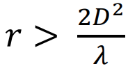
The first requirement is satisfied when the distance from the antenna, r, is both—
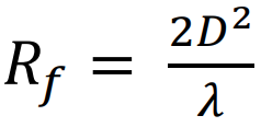
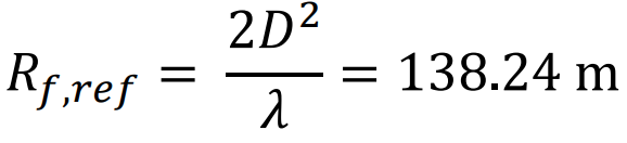
a- greater than the far-field distance 𝑅𝑓 = 2𝐷2÷𝜆 ,where 𝜆 is the wavelength and D is the largest dimension of the antenna, and
b- much greater than 𝜆.
When 𝐷 is more than two or three wavelengths, if 𝑟 > 2𝐷2÷𝜆 then the requirement 𝑟 ≫ 𝜆 is automatically satisfied, which is the case in our problem. In this problem, we assume that the reflector antenna is 2.4 meters in diameter and the frequency of interest is 3.6 GHz where the wavelength is 8.3 cm, so the far field distance for the reflector antenna is 𝑅𝑓,𝑟𝑒𝑓 = 2𝐷2÷𝜆 = 138.24 m (1)
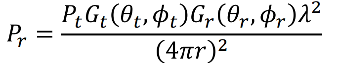
The goal is to determine the power received by a receiver antenna with a gain of 𝐺𝑟(𝜃𝑟 ,𝜙𝑟) where 𝜃𝑟 and 𝜙𝑟 are the offset elevation and azimuth angles with respect to boresight. If the receiver antenna transmits 𝑃𝑡 and has a gain of 𝐺𝑡(𝜃𝑡 ,𝜙𝑡), where 𝜃𝑡 and 𝜙𝑡 are the offset elevation and azimuth angles with respect to boresight of the transmitter, the received power is determined by 𝑃𝑟 = 𝑃𝑡𝐺𝑡 (𝜃𝑡 ,𝜙𝑡 )𝐺𝑟 (𝜃𝑟 ,𝜙𝑟 )𝜆2÷(4𝜋𝑟)2 (2)
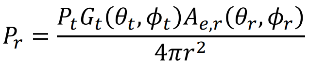
Considering that the effective aperture of antenna – usually a receiving one – is given by 𝐴𝑒 = 𝜆 2𝐺 4𝜋 the above equation can be rewritten as 𝑃𝑟 = 𝑃𝑡𝐺𝑡 (𝜃𝑡 ,𝜙𝑡 )𝐴𝑒,𝑟 (𝜃𝑟 ,𝜙𝑟 ) 4𝜋𝑟 2 where 𝐴𝑒,𝑟 (𝜃𝑟 ,𝜙𝑟 ) = 𝜆 2𝐺𝑟 (𝜃𝑟,𝜙𝑟 ) 4𝜋 is the effective aperture of the receiving antenna in the (𝜃𝑟 ,𝜙𝑟 ) direction.
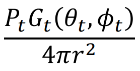
On the other hand 𝑃𝑡𝐺𝑡 (𝜃𝑡 ,𝜙𝑡 ) 4𝜋𝑟 2 is the power density of the radiation at the (𝜃𝑡 ,𝜙𝑡 ) direction usually denoted by 𝑆𝑡(𝜃𝑡 ,𝜙𝑡).
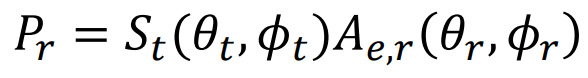
Hence eq. (2) can be rewritten as 𝑃𝑟 = 𝑆𝑡(𝜃𝑡 ,𝜙𝑡)𝐴𝑒,𝑟 (𝜃𝑟 ,𝜙𝑟 ) (3) 11
As it is seen in Figure 1, the transmitting antenna in our problem is a cellular antenna whose radiation pattern is usually omnidirectional, meaning that its gain is not dependent on 𝜙𝑡 . This is usually achieved by using several sector antennae each of them covering a region. To be conservative, we assume that the receiving antenna is at the boresight of the transmitting antenna, making 𝜃𝑡 = 0, and thus maximizing 𝑆𝑡 .
In a coordinate system placed at the center of the receiving antenna with the z-axis in the direction of the cellular antenna, shown by the dashed line in Figure 1, the gain of the receiver antenna, and thus 𝐴𝑒,𝑟 (𝜃𝑟 ,𝜙𝑟 ), is maximum for , 𝜃𝑟 = 0. Assuming a symmetric center-fed antenna, the gain is not dependent on 𝜙𝑟 .
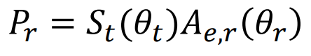
So eq. (3) is reduced to 𝑃𝑟 = 𝑆𝑡(𝜃𝑡)𝐴𝑒,𝑟 (𝜃𝑟 ) (4)
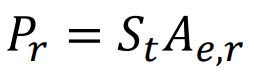
When the boresight of both antennas lie on the dashed line in Figure 1 and 𝜃𝑡 = 𝜃𝑟 = 0, Eq (4) simply reduces to 𝑃𝑟 = 𝑆𝑡𝐴𝑒,𝑟 (5) where 𝑆𝑡 and 𝐴𝑒,𝑟 and maximum values of 𝑆𝑡(𝜃𝑡) and 𝐴𝑒,𝑟 (𝜃𝑟 ) respectively.
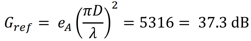
Assuming an aperture efficient, 𝑒𝐴, of 65%, the gain of the reflector antenna is calculated as 𝐺𝑟𝑒𝑓 = 𝑒𝐴 ( 𝜋𝐷 𝜆 ) 2 = 5316 = 37.3 dB 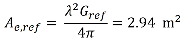 The effective aperture, 𝐴𝑒,𝑟𝑒𝑓, for this reflector antenna is 𝐴𝑒,𝑟𝑒𝑓 = 𝜆 2𝐺𝑟𝑒𝑓 4𝜋 = 2.94 m2
In [5] it is stated that the maximum EIRP of an LTE antenna is 64 dBm per antenna and the gain is 18 dBi, which means that the transmitted power if 46 dBm or 40 W.
The size of a cellular sector antenna at 3.6 GHz will be smaller than the size of our reflector, leading to a smaller far field boundary distance at the same frequency according to 𝑅𝑓 = 2𝐷2 ÷𝜆 . So whenever the farfield criterion for the C-band terminal is satisfied it is also satisfied for the sector antenna.
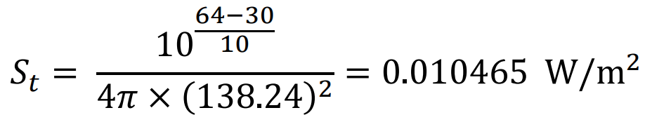
Assuming both antennas are at the boresight of each other, the power spectral density of the cellular antenna at the position of the reflector antenna is computed as follows: 𝑆𝑡 = 10 64−30 10 4𝜋 × (138.24) 2 = 0.010465 W/m2

The power received by the reflector antenna is computed by 𝑃𝑟 = 𝑆𝑡𝐴𝑒,𝑟𝑒𝑓 = 0.010465 × 2.94 = 0.03076 W = 14.9 dBm
These boresight-to-boresight interference levels are summarized in Table 1.
It is worth noting that this level of interference assumes that both antennas are in the boresight of each other which is an extremely unlikely scenario. It also assumes that they are in the closest far-field distance of each other. This scenario was analyzed to gain an understanding of the worst interference in the farfield region. In a more likely scenario, the cellular antenna would be away from the boresight of the Cband terminal by for example 10 degrees that is 𝜃𝑟 = 10 deg. An FCC-compliant terminal cannot have a gain of more than 7 dB which, for our C-band terminal, means about a 30 dB gain reduction from boresight. In this scenario the interference power would be approximately -15 dBm. Some C-band operators have mentioned similar values as what they prefer the tolerance level of the LNB would be.
Interferer at the Near Field Region of the VSAT Terminal
If the distance to the reflector antenna is smaller than 𝑅𝑓,𝑟𝑒𝑓 = 2𝐷2 ÷𝜆 = 138.24 m, the far field approximations do not apply, and one must use different solutions. Phase front and reactive fields are two issues to be considered.
Determining the Power Received by the VSAT Terminal Caused by a 5G Interferer at its Near Field
In this section we determine the power received by the C-band VSAT terminal when the 5G interference is at its near field.
At this distance, it is assumed that the C-band terminal is in the far-field region of the cellular sector antenna. A direct solution would be to compute the power density caused by the cellular antenna and then calculate the received power by the satellite terminal. Unfortunately, since we are in the near field of the satellite terminal, we cannot use the far-field approximations to quickly compute the received power. The method described in [3], presents a way for predicting the power density when the parabolic antenna itself is radiating 𝑃𝑡 . Assuming the far-field conditions for the cellular antenna one can easily determine the power received by the cellular antenna, 𝑃𝑟 . Then the reciprocity theorem is used in this passive system to conclude that if the cellular antenna was transmitting 𝑃𝑡 , the parabolic antenna would receive the same 𝑃𝑟 . So instead of starting from the interferer and going to the receiver we will start from the receiver as if it were the transmitter and we calculate the power received by the cellular antenna.
However, we digress in this paragraph to point out the fact that the cellular antennas are usually an array of patch antennas and hence their far-field criterion is only about the phase front. If the distance is smaller than their far field, the actual gain will be smaller than the far-field gain and hence our computations from this point on will be even more conservative.
The cellular antenna has a gain of 18 dBi and transmits about 40 W [5].
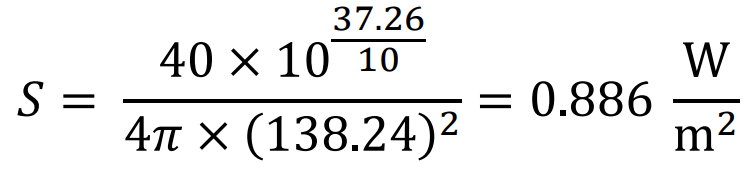
We assume that the reflector antenna is transmitting 40 W. At its far-field distance i.e. at 138.24 m, the power density is 𝑆 = 40 × 10x37.26÷10 ÷4𝜋 × (138.24) 2 = 0.886 W÷m2
According to [3], the strongest power density in the near field on boresight happens when the distance from the antenna is one tenth of the far-field distance and will be about 43 times stronger than the power density on the boresight at the far-field distance. So the highest near field power density will occur at 13.8 m and will equal 43*0.886=38.1 W/m2.
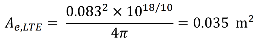
The next step is to determine the power input to the cellular antenna which has an effective aperture of 𝐴𝑒,𝐿𝑇𝐸 = 0.0832 × 10¹⁸/10÷4𝜋 = 0.035 m2
The power input to the cellular antenna is 0.035 × 0.886 = 1.33 W = 31.23 dBm.
Using the reciprocity theorem, one can conclude that if the 40 W was being transmitted at the cellular antenna, the reflector antenna would receive the same 31.23 dBm.
References
[1] ITU-R, Recommendation ITU-R M.2083-0 IMT Vision – Framework and overall objectives of the future development of IMT for 2020 and beyond, 2015.
[2] Huawei Technologies Co LTD; 5G Spectrum - Public Policy Position, 2018
[3] A. Farrar and E. Chang, Procedures for Calculating Field Intensities of Antennas, Figure 4-2(b), 1987
[4] Herbert K. Kobayashi, Procedure for Calculating the Power Density of a Parabolic Circular Reflector Antenna, Fig 3-9(b), 1990
[5] National Telecommunications and Information Administration, “LTE (FDD) Transmitter Characteristics” https://www.ntia.doc.gov/files/ntia/meetings/lte_technical_characteristics.pdf, accessed February 2019.